Training PennyLane Circuits with Keras 3 Multi-Backend

This demo is featured on the PennyLane Community Demos page!

You can find the KerasCircuitLayer in the pennylane-keras3-layer package. (See PyPi link above)

Training PennyLane Circuits with the Keras 3 Multi-Backend

While PennyLane does not support the qml.KerasLayer api since the transition from Keras 2 to Keras 3, we can still define a custom keras layer with certain modifications to allow for integration into keras models. Additionally, due to the multibackend support in Keras 3, these models can be trained using jax, pytorch or tensorflow. This demo will create a Keras 3 implementation of the Data-ReUploading models from the ‘Quantum models as Fourier series ‘ demo.

In case its not installed already, go ahead and install keras and tensorflow. By default the pip package contains Keras 3. For further instructions you can look at this page. Remember to install CUDA enabled versions if you want GPU support. Select which backend you want to install. Its better to have them in separate environments We start by selecting our Keras 3 backend using the ‘KERAS_BACKEND’ environment variable.

import os
os.environ["KERAS_BACKEND"] = "jax" # This can be either JAX, tensorflow, or torch. (tensorflow by default)

We can now import keras alongside its key modules ops. We then print the current backend to verify if everything loaded correctly.

import keras
from keras import ops
print(f"Keras backend: {keras.backend.backend()}")

In order to ensure numerical stability with quantum circuits set the backend to use float64

keras.backend.set_floatx('float64')
if keras.backend.backend() == "jax":
    print("Setting jax to use float64")
    import jax
    jax.config.update("jax_enable_x64", True)

Importing the supporting packages of numpy and matplotlib, alongside PennyLane.

NOTE: Remember to install PennyLane with cuda for GPU support

import pennylane as qml
import numpy as np
import matplotlib.pyplot as plt

Goal of this demonstration

The main goal of this demo is to allow people to integrate PennyLane circuits into their existing code bases. The Keras Layer created here will fully support models saving/loading, training and everything else you normally expect from a Keras Layer. Additionally, they will be entirely self contained, not requiring Qnodes to be defined externally.

In order to get better background on the concepts employed in this demo, here are some helpful additional resources:

• Keras custom layer documentation
• Pennylane QNode documentation
• Keras 3 Pytorch Example

  Setting up the target dataset

Similiar to the [fourier series demo]((https://pennylane.ai/qml/demos/tutorial_expressivity_fourier_series) mentioned in the introduction, we first define a (classical) target function which will be used as a “ground truth” that the quantum model has to fit. The target function is constructed as a Fourier series of a specific degree.

degree = 1  # degree of the target function
scaling = 1  # scaling of the data
coeffs = [0.15 + 0.15j] * degree  # coefficients of non-zero frequencies
coeff0 = 0.1  # coefficient of zero frequency


def target_function(x):
    """Generate a truncated Fourier series, where the data gets re-scaled."""
    res = coeff0
    for idx, coeff in enumerate(coeffs):
        exponent = np.complex128(scaling * (idx + 1) * x * 1j)
        conj_coeff = np.conjugate(coeff)
        res += coeff * np.exp(exponent) + conj_coeff * np.exp(-exponent)
    return np.real(res)

Plotting the ground truth we get

x = np.linspace(-6, 6, 70)
target_y = np.array([target_function(x_) for x_ in x])

plt.plot(x, target_y, c="black")
plt.scatter(x, target_y, facecolor="white", edgecolor="black")
plt.ylim(-1, 1)
plt.show()

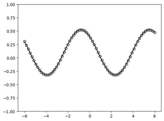Figure 1: Visualization output

Defining the Quantum Model

We first define the quantum model outside the Keras layer for the sake of clarity. We will later encapsulate the entire circuit into our custom Keras Layer.

Note: While we are using the lightning.qubit backend here as an example, this has been tested to work with the lightning.gpu and default.qubit backends as well

dev = qml.device("default.qubit", wires=1) # Define the device for circuit execution

The quantum model consists of a set of repeated trainable unitaries $W(\theta)$ and data encodings via the $S(x)$ function. Additionally, a scaling parameter is used to change the period of the final learned function w.r.t the input data $x$.

scaling = 1.0

def S(x):
    """Data-encoding circuit block."""
    qml.RX(scaling * x, wires=0)


def W(theta):
    """Trainable circuit block."""
    qml.Rot(theta[0], theta[1], theta[2], wires=0)


@qml.qnode(dev)
def serial_quantum_model(weights, x):

    for theta in weights[:-1]:
        W(theta)
        S(x)

    # (L+1)'th unitary
    W(weights[-1])

    return qml.expval(qml.PauliZ(wires=0))

We can now define numpy arrays for the weights and input to draw the circuit in terms of the number of layers (or number of repetitions).

layers = 2  
weights = (
    2 * np.pi * np.random.random(size=(layers + 1, 3))
)  # some random initial weights

Drawing our the quantum circuit for our model

qml.draw_mpl(serial_quantum_model)(weights,1)

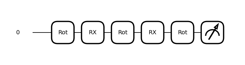Figure 2: Visualization output

Plotting the output of this random circuit, we get

x = np.linspace(-6, 6, 70)
random_quantum_model_y = [serial_quantum_model(weights, x_) for x_ in x]

plt.plot(x, random_quantum_model_y, c="blue")
plt.ylim(-1, 1)
plt.show()

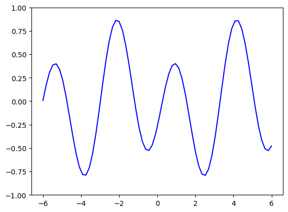Figure 3: Visualization output

Wrapping the QNode in a Keras Layer

You can refer to the full tutorial on creating custom keras layer here. We will now create a custom keras layer can wrap the quantum circuit and its trainable weights. When doing this we have to keep in mind the following Keras 3 specifics:

1. Do not use any tf.xx functions, and only use the native ops.xxx package. For example use ops.sum() rather than tf.reduce_sum or torch.sum.
2. Do not create tf.constant or tf.variables, rather use the self.add_weight method.
3. You need to pass the weights as arguments to the QNode and not use self.weight inside the QNode. In order to fully support model saving, we need to import the following keras functions and mark the layer as serializable. More details about these functions can be found here.

from keras.utils import register_keras_serializable
from keras.saving import serialize_keras_object, deserialize_keras_object

Methods to implement for a custom layer

To create a fully functional keras layer, the following methods need to be implemented

1. __init__ method:

The __init__ method is used to accomplish the following:

• Create the instance variables that define the QNode such as number of wires, circuit backend, etc.
• Create the instance variables that define the circuit such as number of layers
• Select the PennyLane interface based on keras backend to be [“tf”,”torch” or “Jax”]
• Call the super().__init__(**kwargs) to pass generic layer properties such as ‘name’ to the parent class __init__ function.

2. build() method:

The build() method is used to instantiate the model weights at runtime based on input_shape. This can be used to create dynamic circuits with qubits equal to the number of input variables. However in this demo we are ignoring the input shape. Weights are created using the add_weight method, which you can read more about here.

Note: DO NOT apply any operations on the created weight here as it will cause issues with gradients

3. compute_output_shape() method:

This method is required in order to support model.summary() and model.save() functionality. This can be trivially implemented by passing an output_shape parameter in the __init__ method similar to the depricated qml.KerasLayer, or we can implement circuit specific logic. In this example, our circuit outputs a single expectation value per input variable, therefore the output shape is ‘(batch,num_of_wires)’

4. QNode methods:

The ‘QNode’ methods consist of 2 sets of methods -

1. Circuit Definition Methods : These methods create the QNode circuit structure and can be implemented as a single method or a set of methods which implement different sub-circuits. Here we use 2 sub-circuit methods self.W and self.S, along with the self.serial_quantum_model method to define the final structure and returned measurements.
2. Circuit Creation Method : This method defines the PennyLane device and the QNode from the circuit definition as an instance variables.

Note: Pennylane requires the input to be the last argument to properly work with batched inputs

5. call() method:

The call() methods needs to call the Qnode with the weight variable. Additional pre-processing can be applied before calling the circuit as well, for example we apply input variable scaling outside the circuit to take advantage of efficient vectorized execution for batched input. Depending on your specific model, we can also include pre-processing steps such as input scaling. Due to being wrapped by the autodiff of the various backends, we will still get valid gradients for these steps.

6. draw_qnode method:

A Utility methods to plot the QNode circuits

7. get_config method:

This method needs to be implemented to support model.save functionality. It creates a config(dict) which defines the configuration of the current layer.

Note: While scalar data such as int, float and str, do not need the serialize_keras_object function, it is typically good practice to wrap all the parameters using this method.

8. from_config method:

This method needs to be implemented to support model.save functionality. It defines how to create an instance of the layer from a configuration.

JAX Specific Adaptations:

When using the jax backend, pennylane circuits are automatically compiled with jax.jit. This includes the device creation for randomness support. The forward pass then needs to support call the .value on the keras variable for support with the jax compiled circuit

@register_keras_serializable(package="QKeras", name="QKerasLayer")
class QKerasLayer(keras.layers.Layer):
    def __init__(self,layers:int,
                 scaling:float=1.0,
                 circ_backend="lightning.qubit",
                 circ_grad_method="adjoint",
                 num_wires:int=1,
                 use_jax_python:bool = False, 
                 **kwargs):
        """A Keras Layer wrapping a PennyLane Q-Node.
        Args:
            layers (int): Number of layers in the DR Model. 
            circ_backend (str): Backend for the quantum circuit. Defaults to 'lightning.qubit'
            circ_grad_method (str): Gradient method for the quantum circuit. Defaults to 'adjoint'
            num_wires (int): Number of wires to iniatize the qml.device. Defaults to 1.
            scaling (float): Scaling factor for the input data. Defaults to 1.0
            use_jax_python (bool): Flag to use the vectorized jax backend. NOTE: This does not support jax.jit compilation see: https://docs.pennylane.ai/en/stable/introduction/interfaces/jax.html for details
            **kwargs: Additional keyword arguments for the keras Layer class such as 'name'.
        """
        super().__init__(**kwargs) # Passing the keyword arguments to the parent class 
        # Defining the circuit parameters
        self.layers = layers
        self.scaling = scaling
        self.circ_backend = circ_backend
        self.circ_grad_method = circ_grad_method
        self.num_wires = num_wires
        
        # Define Keras Layer flags
        self.is_built : bool = False
        
        # Selecting the Pennylane interface based on keras backend
        if(keras.config.backend() =="torch"):
            self.interface = "torch"
        elif(keras.config.backend() =="tensorflow"):
            self.interface = "tf"
        elif(keras.config.backend() =="jax"):
            if(use_jax_python):
                self.interface = "jax-python"
            else:
                self.interface = "jax"
    
    def build(self,input_shape):
        """ Initialized the layer weights based on input_shape
        Args:s
            input_shape [tuple]: The shape of the input 
        """
        # Save input_shape without batch to be used later for the draw_circuit function  
        self.input_shape = input_shape[1:]
        
        ## We initialize weights in the same way as the numpy array in the previous section.
        # Randomly initialize weights to uniform distribution in the a range of [0,2pi)
        self.layer_weights = self.add_weight(shape=(self.layers+1,3),initializer = keras.initializers.random_uniform(minval=0,maxval=2*np.pi),
                                             trainable=True) 
        
        # Create Quantum Circuit
        self.circuit = self.create_circuit()
        
        # Set the layer as built
        self.is_built = True
        
    def compute_output_shape(self,input_shape):
        """ Return output shape as a function of the input shape"""
        # For this model we return an expectation value per qubit. The '0' index of the input_shape is always the batch, so we return an output shape of (batch, num_wires)
        return (input_shape[0],self.num_wires)

    ## We define the subcircuit functions for the circuit.
    def S(self,x):
        """Data-encoding circuit block."""
        # Use the [:,0] syntax for batch support 
        qml.RX(x[:,0], wires=0)
    
    def W(self,theta):
        """Trainable circuit block."""
        qml.Rot(theta[0], theta[1], theta[2], wires=0)

    ## Define the QNode code as a class method **without qml.qnode decorator**
    def serial_quantum_model(self,weights, x):
        """ Data Re-Uploading QML model"""
        for theta in weights[:-1]:
            self.W(theta)
            self.S(x)
    
        # (L+1)'th unitary
        self.W(weights[-1])
        return qml.expval(qml.PauliZ(wires=0))
 
    def create_circuit(self):
        """ Creates the PennyLane device and QNode"""
        if self.interface == "jax":
            @jax.jit
            def create_circuit_jax_jit(layer_weights, x):
                dev = qml.device(self.circ_backend, wires = self.num_wires)
                circuit_node = qml.QNode(self.serial_quantum_model, dev, diff_method=self.circ_grad_method, interface=self.interface)
                return circuit_node(layer_weights, x)
            return create_circuit_jax_jit
        else:
            dev = qml.device(self.circ_backend, wires = self.num_wires)
            return qml.QNode(self.serial_quantum_model, dev, diff_method=self.circ_grad_method, interface=self.interface)
            
    def call(self,inputs):
        """Defines the forward pass of the layer """
        ## We need to prevent the layer from being called before the weights and circuit are built
        if (not self.is_built):
            raise Exception("Layer not built") from None
            
        # We multiply the input with the scaling factor outside the circuit for optimized vector execution. 
        x = ops.multiply(self.scaling, inputs)
        # We call the circuit with the weight variables.
        if(self.interface == "jax"):
            out = self.circuit(self.layer_weights.value, x)
        else:
            out = self.circuit(self.layer_weights, x)
        return out

    def draw_qnode(self):
        """ Draw the layer circuit"""
        ## We want to raise an exception if this function is called before our QNode is created
        if (not self.is_built):
            raise Exception("Layer not built") from None
        ## Create a random input using the input_shape defined earlier with a single batch dim
        x = ops.expand_dims(keras.random.uniform(shape = self.input_shape),0)
        qml.draw_mpl(self.circuit)(self.layer_weights.numpy(), x)

    def get_config(self):
        """ Create layer config for layer saving"""
        ## Load the basic config parameters of the keras.layer parent class
        base_config = super(QKerasLayer, self).get_config()
        ## Create a custom configuration for the instance variables unique to the QNode
        config = {
            "layers": serialize_keras_object(self.layers),
            "scaling": serialize_keras_object(self.scaling),
            "circ_backend": serialize_keras_object(self.circ_backend),
            "circ_grad_method": serialize_keras_object(self.circ_grad_method),
            "num_wires": serialize_keras_object(self.num_wires),
        }
        return {**base_config, **config}

    @classmethod # Note that this needs to be a class function and not an instance method
    def from_config(cls, config):
        """ Create an instance of layer from config"""
        # The cls argument is the specific layer config and the config object contains general keras.layer arguments
        layers = deserialize_keras_object(config.pop("layers"))
        scaling = deserialize_keras_object(config.pop("scaling"))
        circ_backend = deserialize_keras_object(config.pop("circ_backend"))
        circ_grad_method = deserialize_keras_object(config.pop("circ_grad_method"))
        num_wires = deserialize_keras_object(config.pop("num_wires"))
        # Call the init function of the layer from the config
        return cls(layers=layers,
                   scaling= scaling,
                   circ_backend=circ_backend,
                   circ_grad_method=circ_grad_method,
                   num_wires = num_wires, 
                   **config)
        

We can now test out our layer class by initializing it using the same arguments as the previous section

layers = 2  
keras_layer = QKerasLayer(layers = layers,
                          scaling=1.0,
                          circ_backend="default.qubit",
                          num_wires=1,
                          name="QuantumLayer",
                          # Use the flag below to experiment with vectorized jax
                          # use_jax_python=True 
                         )

Integrating the layer in a Keras Model

In order to test the layer functionality, let’s integrate it into a simple keras model

# Simple univariate input layer
inp = keras.layers.Input(shape=(1,))
out = keras_layer(inp)
model = keras.models.Model(inputs=inp,outputs=out,name="QuantumModel")
model.summary()

Looking at the model summary. We can verify if everything looks correct based on -

• The number of trainable parameters - Since our weights are of the shape (layers+1,3), we can expect a shape of (2+1,3) = (3,3) = 9 parameters
• The name of the layer matching what we passed in the instantiation

Model: "QuantumModel"
┏━━━━━━━━━━━━━━━━━━━━━━━━━━━━━━━━━┳━━━━━━━━━━━━━━━━━━━━━━━━┳━━━━━━━━━━━━━━━┓
┃ Layer (type)                    ┃ Output Shape           ┃       Param # ┃
┡━━━━━━━━━━━━━━━━━━━━━━━━━━━━━━━━━╇━━━━━━━━━━━━━━━━━━━━━━━━╇━━━━━━━━━━━━━━━┩
│ input_layer_9 (InputLayer)      │ (None, 1)              │             0 │
├─────────────────────────────────┼────────────────────────┼───────────────┤
│ QuantumLayer (QKerasLayer)      │ (None, 1)              │             9 │
└─────────────────────────────────┴────────────────────────┴───────────────┘

Plotting inner QNode

Integrating the layer into a model and calling the model.summary() function also calls the layer.build function. Therefore our circuit,weights and device should be instantiated. We can verify this calling our draw_qnode helper function to see the circuit plot.

keras_layer.draw_qnode()

Figure 4: Visualization output

keras_layer.layer_weights

We can see the weights of the layer are initialized to random values.

<Variable path=QuantumLayer/variable_9, shape=(3, 3), dtype=float64, 
    value=[[2.67741224 5.22959572 3.46291224]
        [4.48692751 2.2729619  4.06532814]
        [4.69508503 4.24126382 5.68455441]]>

Test forward pass

Similar to earlier, lets test our layer inference by calling the model with the random weights and plotting the outputs.

Note: When using the torch backend, we might need to call the .to(‘cpu’) on the model predictions before we can plot them if the system has a GPU

x = np.linspace(-6, 6, 70)
random_quantum_model_y = model(x)
# Uncomment the following when using the torch backend
# random_quantum_model_y = random_quantum_model_y.to('cpu').detach().numpy()
plt.plot(x, random_quantum_model_y, c="blue")
plt.ylim(-1, 1)
plt.show()

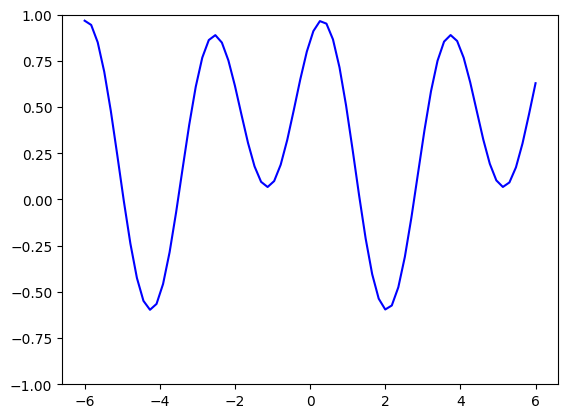Figure 5: Visualization output

Model Training

We can now train the model using the normal keras training functions of model.compile and model.fit.

We will first compile the model with the mean_squared_error loss function and the Adam optimizer

model.compile(optimizer=keras.optimizers.Adam(learning_rate=0.03),
              loss = keras.losses.mean_squared_error,run_eagerly=True)

We can then train the model with the model.fit function for x and target_y.

model.fit(x=x,y=target_y,
          epochs=30)

Epoch 1/30
3/3 ━━━━━━━━━━━━━━━━━━━━ 2s 209ms/step - loss: 0.2158
Epoch 2/30
3/3 ━━━━━━━━━━━━━━━━━━━━ 0s 51ms/step - loss: 0.1636
.
.
.
Epoch 29/30
3/3 ━━━━━━━━━━━━━━━━━━━━ 0s 52ms/step - loss: 8.7295e-04
Epoch 30/30
3/3 ━━━━━━━━━━━━━━━━━━━━ 0s 52ms/step - loss: 8.6801e-04
<keras.src.callbacks.history.History at 0x79bbf42a7ef0>

Plotting the outputs of the trained model against the ground truth

The model should train relatively fast. If your loss is $<10^{-2}$, the fit should be very good

predictions = model(x)
## Uncomment the following line for the torch backend
# predictions = predictions.to('cpu').detach().numpy()

plt.plot(x, target_y, c="black")
plt.scatter(x, target_y, facecolor="white", edgecolor="black")
plt.plot(x, predictions, c="blue")
plt.ylim(-1, 1)
plt.show()

Figure 6: Visualization output

Model Saving and Loading

Due to implementing the get_config and from_config methods, our model should be fully compatible with the keras.save and keras.models.load_model methods.

Saving

Lets first save the trained models. It should save with no errors and create a ‘.keras’ file.

model.save("./model.keras")

Loading

Now lets test model loading and see if we can get the same inference with the loaded model

model2 = keras.models.load_model("./model.keras")

Now plotting the outputs we should see similiar if not identical results

predictions2 = model2(x)
## Uncomment the following line for the torch backend
# predictions2 = predictions2.to('cpu').detach().numpy()
plt.plot(x, target_y, c="black")
plt.scatter(x, target_y, facecolor="white", edgecolor="black")
plt.plot(x, predictions2, c="blue")
plt.ylim(-1, 1)
plt.show()

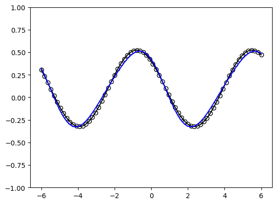Figure 7: Visualization output

Final Notes

Try changing the keras backend variable in the beginning of this demo and see how the process works with a different backend